Marine ecology progress series 353:275

Vol. 353: 275–288, 2008
MARINE ECOLOGY PROGRESS SERIES
Published January 17
doi: 10.3354/meps07164 Mar Ecol Prog Ser
Summer spatial distribution of cetaceans in
the Strait of Gibraltar in relation to
the oceanographic context
Renaud de Stephanis1, 2,*, Thomas Cornulier3, 4, Philippe Verborgh1, 2,
Juanma Salazar Sierra1, 2, Neus Pérez Gimeno2, 5, Christophe Guinet3
1CIRCE, Conservation Information and Research on Cetaceans, C/Cabeza de Manzaneda 3, Algeciras-Pelayo, 11390 Cadiz, Spain
2Sociedad Española de Cetáceos C/Nalon 16, La Berzosa, Madrid, Spain
3Centre d'Études Biologiques de Chizé, CNRS UPR 1934, 79 360 Villiers en Bois, France
4School of Biological Sciences, Zoology Building, Tillydrone Avenue, University of Aberdeen, Aberdeen AB24 2TZ, UK
5Laboratorio de Ingeniería Acústica de la Universidad de Cádiz (LAV), CASEM, Río de San Pedro S/N, Puerto Real, Cádiz, Spain
ABSTRACT: The Strait of Gibraltar, the only passage between the Mediterranean Sea and theAtlantic Ocean, and characterised by a surface inflow of Atlantic waters and a deep outflow ofMediterranean waters, is inhabited by a large number of cetacean species. The present study focuseson the occurrence and the spatial distribution of cetacean species within the strait in relation tooceanographic features. Shipboard visual surveys were conducted during the summers of 2001 to2004, covering 4926 km. A total of 616 sightings of 7 cetacean species were made. The spatial distri-butions of 6 species (short-beaked common dolphins Delphinus delphis, striped dolphins Stenellacoeruleoalba, bottlenose dolphins Tursiops truncatus, long-finned pilot whales Globicephala melas,sperm whales Physeter macrocephalus and killer whales Orcinus orca) were examined with respectto depth and slope. The analyses indicate that these species could be ordered into 3 groups. A firstgroup, with a northward tendency, is composed of common and striped dolphins. Due to its at-sealocation and feeding habits, this group is likely to feed on mesopelagic fishes or squids associatedwith the surface Atlantic waters. The second group, constituted by bottlenose dolphins, long-finnedpilot whales and sperm whales, is mainly found over the deep waters of the central part of the strait.
While the foraging ecology of bottlenose dolphins is still unclear, both sperm whales and pilot whalesare most likely to feed on squids occurring in deep Mediterranean waters. The third group, formedby killer whales Orcinus orca, was associated with blue fin tuna Thunnus thynnus fisheries in thesouthwestern part of the strait.
KEY WORDS: Cetacean · Strait of Gibraltar · Spatial distribution · Feeding ecology · Fisheries interaction Resale or republication not permitted without written consent of the publisher and not the Strait of Gibraltar itself (Aguilar 2006). Asurvey conducted from ferries navigating between Cetacean distribution and abundance in the Strait of Spain and Morocco from March to May 1999 found Gibraltar is poorly described and limited to a few that the main species encountered in the eastern part sources. One of the latter relies on data from commer- of the strait were the striped dolphin Stenella cial whaling activities, which took place between 1921 coeruleoalba, short-beaked common dolphin Delphi- and 1959 from shore-based whaling stations located in nus delphis and, occasionally, bottlenose dolphin Tur- Getares (Spain) and Benzou (Morocco) and from fac- siops truncatus, long-finned pilot whales Globicephala tory ships (Aguilar 2006). But these data describe the melas and sperm whales Physeter macrocephalus situation in the Atlantic areas off the Strait of Gibraltar, (Roussel 1999). Finally, studies from the Spanish drift- Inter-Research 2008 · www.int-res.com Mar Ecol Prog Ser 353: 275–288, 2008 net fishery operating until 1994 in the strait also 6°W in the central part of the strait (Kinder et al. 1988).
revealed the presence of common dolphin and striped This Atlantic–Mediterranean water interface is consid- dolphin (Silvani et al. 1999). In 2005, a study provided ered to be a biogeographic boundary (Sanjuán et al.
evidence of the presence of these species in the 1994). Nevertheless, there is substantial transport of Alborán Sea (Cañadas et al. 2005). However, the rela- organisms across this ecotone. Most of the plankton tive density and the spatial distribution of the cetacean biomass is transported into the Mediterranean Sea by species encountered within the Strait of Gibraltar Atlantic waters. Reul et al. (2002) estimated that 5570 t remain unknown.
C d–1, dominated by autotrophic nanoplankton (42%) The Strait of Gibraltar is the narrow and shallow con- and heterotrophic bacteria (37%), is transported nection between the Mediterranean Sea and the towards the Mediterranean Sea, while 1140 t C of het- Atlantic Ocean (Fig. 1). The water circulation in the erotrophic organisms (89%) is exported daily towards strait is characterised by: (1) a surface inflow of the Atlantic by the deep Mediterranean outflow.
Atlantic waters, which is driven by the excess of evap- The highest biomass concentrations were observed oration over precipitation in this basin, and (2) a deep in the northern part of the strait, where enriched outflow of dense Mediterranean water (Lacombe & Atlantic shelf waters circulate (Van Geen & Boyle Richez 1982). The strait is also characterised by mixing 1988). However, due to higher current velocities, most processes through pulsed upwelling induced by the of the biomass import took place in the central and tides and constrained by the bathymetry of the area southern parts of the strait, where we would expect to (Echevarría et al. 2002).
find high concentrations of cetaceans, as ecological The interface between the Atlantic surface waters studies of apex predators at sea indicate that their dis- and the deep Mediterranean waters generally takes tribution and abundance can often be related to place at a depth between 50 and 200 m, depending on oceanographic features and marine productivity.
the geographic location and intensity of the tidal flows.
Bathymetry plays an important role on prey distribu- The boundary between Atlantic waters and Mediter- tion (Gil de Sola 1993). This role can be direct, as on ranean waters becomes deeper from the Spanish coast demersal prey, for which the distribution can often be to the Moroccan coast (north to south) (Reul et al. 2002) related to topographic features such as depth and and from the Atlantic to the Mediterranean (east to slope. For pelagic cetacean prey species, such as fishes west), from approximately 100 m at 5° 20' W to 300 m at or cephalopods, bathymetric features could act indi- Fig. 1. Study area and bathymetry of the Strait of Gibraltar de Stephanis et al.: Summer distribution of cetaceans in the Strait of Gibraltar rectly through topographically induced vertical (up- MATERIALS AND METHODS
welling) and horizontal (currents) circulation, both ofwhich can stimulate the primary and secondary pro- Study area and surveys. The study area encom-
duction, but could also act directly on the spatial distri- passes the Strait of Gibraltar and its contiguous waters, bution of prey species through transport and/or aggre- between 5 and 6°W, including Spanish and Moroccan gating effects (Davis et al. 1998, Cañadas et al. 2005).
waters. The Strait of Gibraltar (Fig. 1) is nearly 60 km Modelling the relationships between cetacean distri- long. Its western border is located between Cape bution and environmental factors is a complicated task Trafalgar (Europe) and Cape Espartel (Africa), 44 km for several reasons. For instance, relationships be- apart. The strait then narrows to the east to reach a tween cetacean abundance and habitat features may minimum width of 14 km between Tarifa (Europe) and be non-linear. To overcome this problem, many Punta Cires (Africa). Its eastern border is located cetacean distribution studies have used generalised between Gibraltar and Punta Almina (Africa), 23 km additive models (GAMs) that can fit non-parametric apart. The bathymetry of the strait is characterised by smoothing functions of the data (see e.g. Forney 2000, a west to east canyon, with shallower waters (200 to Redfern et al. 2006, Williams et al. 2006).
300 m) found on the Atlantic side and deeper waters More importantly, cetacean surveys rarely follow (800 to 1000 m) on the Mediterranean side (Fig. 1).
systematic designs in space and time, due to specific Survey transects were conducted from the CIRCE logistical constraints, especially when conducted from (Conservation, Information and Research on Ceta- opportunistic platforms (Williams et al. 2006). There- ceans) research motorboat ‘Elsa' (11 m length), sam- fore, sampling effort is typically heterogeneous and pling the study area throughout the months of July, needs to be carefully accounted for (Redfern et al.
August and September between 2001 and 2004. Tran- 2006). Additionally, encounter rates with cetaceans are sects were conducted without any pre-defined track often very low, typically resulting in sparse data that for each of these surveys, but they were designed to are difficult to analyse, both in terms of abundance and cover the whole range of bathymetry in the strait probability of sighting. The problem is even more every month by crossing the isobaths perpendicularly.
acute with species living in (potentially large) groups While carrying out the surveys it was attempted to that tend to generate extremely skewed or over- maximise the presence at sea, with restrictions due dispersed distributions of counts for which standard to the maritime traffic present in the area and the (e.g. binomial, Poisson, or log-normal) statistical mod- meteorological conditions. The sampling strategy was els may not be suitable.
constant throughout the survey period. The area Additionally, animal distribution data are autocor- was surveyed at an average speed of 5.6 knots related, especially for organisms like cetaceans, which (9.8 km h–1). Searching effort stopped when a group live in schools. Accounting for spatial autocorrelation is of cetaceans was approached and started again when vital when modelling the relations between animal the sighting was ended, with a return to the course distribution and the environment (Keitt et al. 2002).
Although this restraint is recognised in cetacean litera- The observers were placed on an observation plat- ture, a recent review of this field suggests that very form, 4 m above the sea level. Two trained observers few, if any, studies have attempted to include spatial occupied the observation lookout post in 1 h shifts dur- correlation in cetacean–habitat models (Redfern et ing daylight, with visibility over 3 nautical mile (5.6 km), assisted with 8 × 50 binoculars, covering 180° In the present paper we propose to deal with these ahead of the vessel. Sighting effort was measured as issues within a single model-based approach. In accor- the number of kilometres travelled with adequate dance with, e.g., Williams et al. (2006), we use GAMs, sighting conditions (i.e. with a sea state Douglas of < 4 while paying careful attention to controlling for error and 2 observers at the lookout post. The Douglas sea dispersion by using quasi-binomial methods (for pres- state estimates the sea's roughness for navigation.) ence/absence data). In addition, we show that spatial The geographic position of the ship was recorded autocorrelation can be included explicitly in order to every minute on the ship's computer from a GPS select more parsimonious cetacean–habitat models.
(global positioning system) navigation system logger Our study focuses on the summer cetacean distribu- using the IFAW (International Fund for Animal Wel- tions in the Strait of Gibraltar with the aims: (1) to esti- fare) Data Logging Software Logger 2000, Version 2.20 mate the relative abundance of cetacean species, (2) to investigate how their distribution is related to the ?oid=25739). Data concerning the location and time of bathymetric features of the Strait of Gibraltar and (3) to a sighting and the species, number of individuals and examine the inter-specific spatial association in the behaviour were recorded along with ancillary environ- Strait of Gibraltar in summer.
mental data (sea state, wind speed, visibility). These

Mar Ecol Prog Ser 353: 275–288, 2008 environmental data were also taken every 20 min, and 100, where Ind is the number of individuals of a given at every course change of the boat.
species observed versus effort in the research area, According to the Sociedad Española de Cetaceos including only sightings when the animals were (SEC 1999), a sighting was defined as a group of ani- approached, and Eff is the distance (km) covered ver- mals of the same species seen at the same time, show- ing similar behaviour and for which the maximum dis- Spatial distribution and bathymetry. The encounter
tance between 2 individuals was <1000 m. When a rate for each species was calculated for each quadrat group of animals was first seen, the location of the ship, using the number of sightings per species per 100 km and the distance and bearing of the cetaceans were searched, pooled over the 4 yr of the study. Only sight- recorded, to be able to localise the animals when ings for which approach was established (i.e. the ani- approaching them. The location of the animals was mals' location was within a 100 m radius of the boat's also recorded when they had been approached by the GPS position) were used for these analyses because vessel (i.e. <100 m away). Eighty-eight groups of some species, like sperm whales, are visible several cetaceans were sighted, but not all were approached kilometres away from the survey track and conversely (see Table 1). The observation effort did not take into could not be located precisely.
account the kilometres sailed while tracking the Two bathymetric features were assessed: the depth and the slope. Mean depth and slope were calculated The study area was divided into quadrats, with a cell for each quadrat. Depth was obtained from the resolution of 2 min latitude (3704 m) by 2 min longitude ETOPO2v2 global elevation data set (2' × 2'); mean (3006 m) (Fig. 2). This scale was used to be able to com- depth (range from 0 to 850 m) was calculated for each pare these results with results gathered in future quadrat. The bathymetric gradient was defined as the research programs carried out by members of the maximum slope around each pixel from the local Spanish Cetacean Society. The distance in kilometres slopes in x and y. Only neighbours above, below, left searched in each quadrat was calculated using a Geo- and right of the pixel are accounted for in this ‘rook's graphic Information System: Arc View 3.2 from ESRI case procedure', and the largest value was kept. The and its extension Animal Movement (Hooge & Eichen- algorithm IDRISI Module Surface Analysis computes laub 2000). Only cells with sighting effort of at least the percent slope for each pixel using the ‘tangent' 3 km were used for the analysis (Fig. 2).
trigonometric function. Slope values were expressed in Presence of cetaceans and relative abundance. Two
metres per kilometre and ranged from a minimum of 0 parameters were defined to quantify cetacean relative to a maximum of 240 m km–1. Analyses of distribution abundance. (1) The encounter rate (ER) is the number of cetaceans according to depth and slope were made of sightings of a given species per 100 km and is based on a continuous depth and slope data set (i.e. the defined as: ER = (Sigh/Eff) × 100, where Sigh is the mean values of quadrats), but depth and slope were number of sightings made of a species versus effort in ranked into subjective depth and slope categories to the research area, including all sightings whether the provide a pertinent ecological context for the interpre- animals were approached or not, and Eff is the dis- tation of the results (Figs. 3 & 4). The depth was cate- tance (km) covered versus effort. (2) The abundance gorised according to the diving capabilities of the rate (AR) (ind. 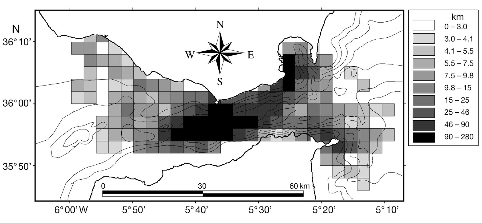km–1) was defined as: AI = (Ind/Eff) × cetaceans observed in this study: 0 to 200 m (reachable Fig. 2. Distribution of the observa-tion effort in kilometres spent by quadrat over the study area de Stephanis et al.: Summer distribution of cetaceans in the Strait of Gibraltar Delphinus delphis Orcinus orca Fig. 3. Distribution of encounter rate (bars) and effort in kilometres (r) in relation to depth Delphinus delphis Orcinus orca Fig. 4. Distribution of encounter rate (bars) and effort (r) in relation to slope by all species), 200 to 600 m (typical depth of long- ture in the model. The 2 covariates used were the con- finned pilot whales) and > 600 m (reachable mostly by tinuous measures of depth and slope, which were sig- sperm whales). The slope was categorised following nificantly correlated in this data set (n = 141, r = 0.23, the categories of Piatt et al. (2006) as gentle (0 to 80 m p = 0.005). However, this correlation was sufficiently km–1), moderate (80 to 160 m km–1) and steep (160 low to justify including both covariates in the models.
to 240 m km–1).
The degree of smoothing for the non-linear terms was The relationships between species probability of selected as part of the model fitting procedure using presence, encounter rates and environmental variables the default generalised cross-validation method (GCV) were investigated using generalized additive mixed implemented in the ‘gamm' function (Wood 2006). As effects models (GAMMs), using the ‘gamm' function of for correlation structure, we used both the exponential the ‘mgcv' library (Wood 2006) in R 2.4.1 (R Develop- model [the correlation between 2 points the distance r ment Core Team 2006). Smooth terms were used in apart is modelled as: (1 – n) × exp(–r/d), where d is the order to allow for non-linear responses to the covari- range and n is the nugget effect, i.e. the correlation at ates, and spatial autocorrelation was accounted for by distance 0 and r is the Euclidian distance], and the including a spherical or exponential correlation struc- spherical model {correlation is modelled as: (1 – n) × [1 Mar Ecol Prog Ser 353: 275–288, 2008 – 1.5(r /d) + 0.5(r /d)3], and takes the value 0 if r × d}, as using 2 indices of the frequency of co-occurrence: the implemented by the ‘corExp' and ‘corSpher' functions half-weight association index and the simple ratio of the ‘nlme' library for mixed-effect models in R (Pin- association index (Ginsberg & Young 1992). However, heiro & Bates 2000). The range is the distance until 2 as the inferences drawn were the same for the 2 observations are correlated. Beyond this distance, they indices, only values of the half-weight association are considered independent. The nugget is the corre- index will be presented. Species present in the same lation at a distance near zero. Variograms were esti- quadrat were considered associated for this quadrat.
mated using defaults of the function, i.e. using 50 dis- To illustrate the association patterns of the species, tance lags covering the whole range of distances in the average-linkage cluster analyses (Manly 1994) were study area. The spherical and exponential models are constructed (see Fig. 12). We used permutation tests among the most versatile and commonly used correlo- (Bejder et al. 1998) to test whether the association pat- gram models and proved satisfactory in all the situa- terns of the observed species were different from what tions we encountered; therefore, no other model was might be expected at random. An observed standard tried. The choice between the 2 types of correlation deviation of the pairwise association indices that is sig- structures was based on minimising the deviance of nificantly larger than those from permuted data sets is the models and by visually checking the variogram.
taken as evidence that species share or avoid the When the exponential and spherical models gave quadrates with other species (Bejder et al. 1998). All indistinguishable results, the spherical was chosen quadrats were included; 20 000 permutations were because of its range parameter (i.e. the distance generated for each test; and to ensure that p-values beyond which 2 observations are independent) has a were stable, 6 runs of the permutation test were gener- more intuitive interpretation. We did not attempt to ated using the simple ratio and half-weight association include any anisotropy in the spatial correlation struc- indices in 3 runs each.
ture because: (1) anisotropic correlograms are not cur- Boat distribution. The distribution of blue fin tuna
rently implemented in the ‘nlme' library (Pinheiro & Thunnus thynnus fishing boats was assessed to test if it Bates 2000) used for the spatial component of the was related to the distribution of cetacean species.
GAMMs and (2) it is reasonable to assume that the Every 20 min, a sampling station was established only likely source of anisotropy in this data set would during the surveys, and tuna boats fishing within be related to the east –west orientation of the Strait of 1 mile were counted. If there was a doubt regarding Gibraltar's topography, which is already accounted for the distance, a Radar JRC 1000 was used to estimate by our covariates (depth and slope).
the distance of the boats. The type of fishing boat was For all species, a large number of grid cells had ER confirmed using binoculars. The mean number of tuna equal to zero. Quasi-binomial GAMM was used after boats was then calculated in each quadrat where converting into presence/absence data. Quasi-bino- at least 5 sampling stations had been conducted mial models are logistic regressions (binomial error) (results see Fig. 11).
allowing for under- or over-dispersion. Because ERwas more variable in less intensively surveyed cells,observation effort per cell (in km) was included as a covariate, assuming that the probability of sighting aspecies in a given cell is proportional to the observa- Search effort in the research area
tion effort. Model selection was based on a forwardselection approach. Covariates were retained in the A total of 6332 km of transect were covered in the model when the associated coefficient was signifi- research area during the months of July, August and cantly different from zero.
September 2001 to 2004. Of those, 4926 km were sur- For the species with the largest number of sightings veyed during the effort transects. They encompassed (common dolphin and striped dolphin), we repeated 150 quadrats, which represent 1670 km2 (Fig. 2).
the models on a yearly basis in order to check if therelation to environmental covariates differed from oneyear to another. For the other species, the numbers of Cetacean presence and relative abundance
quadrats with recorded presence were too few peryear to expect reliable results: bottlenose dolphin A total of 606 sightings of 7 species were recorded (in (maximum number of quadrats in which presence was 24 of which the species could not be identified) within recorded in one given year = 8), pilot whale (12), killer the research area on effort, and were thus used for the whale (4) and sperm whale (11).
calculation of the general ER. In 518 sightings (in 4 of Overlap in distribution. The strength of the spatial
which the species could not be identified), the ceta- relationships between pairs of species was represented ceans were approached, and these sightings were de Stephanis et al.: Summer distribution of cetaceans in the Strait of Gibraltar used to calculate the ER and AR in each quadrat linear effect of observation effort and slope on the (Table 1). Mean numbers of individuals in the groups dolphin's probability of presence in a cell, and no for each species are given in Table 1. Fig. 2 shows the significant effect of the depth (Table 2). We repeated distribution of the encounter rates with respect to the the quasi-binomial models on a yearly basis, assuming depth. In terms of sightings, the most commonly a linear effect of each covariate in order to obtain observed species were the sperm whale Physeter parametric coefficients. Depth did not appear sig- macrocephalus and the long-finned pilot whales Glo- nificant in any year, and the slope had a significant bicephala melas. The less commonly observed species positive effect in 2001 (0.011 ± 0.004, p = 0.01, were the fin whale Balaenoptera physalus, with only 3 Napproached = 32, Nsurveyed = 119), 2002 (0.030 ± 0.011, sightings, and the killer whale Orcinus orca (Table 1).
p = 0.005, Napproached = 19, Nsurveyed = 80), but not in 2003 When the mean number of individuals present within a (0.012 ± 0.012, p = 0.32, Napproached = 6, Nsurveyed = 81) or group is taken into account, the most abundant species 2004 (–0.001 ± 0.014, p = 0.93, Napproached = 4, Nsurveyed = were the striped dolphin Stenella coeruleoalba and the 47), which is most likely a result of insufficient sta- common dolphin Delphinus delphis, while the less tistical power.
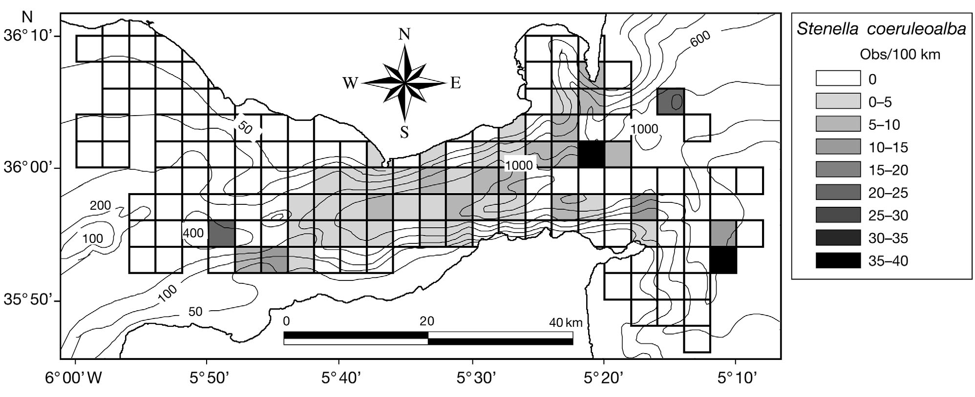
commonly seen species were the fin whale and the Striped dolphins Stenella coeruleoalba were ob- sperm whale (Table 1).
served in 32.7% of the quadrats sampled (Fig. 6). Thespecies presence was positively and linearly related tothe observation effort, the depth and the slope of the Distribution in relation to bathymetric features
sea bottom (suggesting that striped dolphins occur inthe deepest and steepest parts of the strait) (Table 2).
Due to their low ER, fin whales were excluded from The quasi-binomial models were fitted again on a these analyses. The distribution of the ER, with respect yearly basis, assuming, in turn, a linear effect of depth to the effort in each interval of depth and slope for the and slope. Depth had a significant positive effect on 6 most commonly seen species of cetaceans is shown in the probability of presence in 2001 (0.004 ± 0.001, p = Figs. 3 & 4. The spatial distribution of their ER is 0.0003, Napproached = 32, Nsurveyed = 119) and 2004 (0.006 presented in Figs. 5 to 10. The analyses of the spatial ± 0.003, p = 0.039, Napproached = 9, Nsurveyed = 47), but distribution of cetacean species within the strait are not in 2002 (–0.001 ± 0.002, p = 0.60, Napproached = 24, summarised in Table 2.
Nsurveyed = 80) or 2003 (–0.0003 ± 0.002, p = 0.88, Common dolphins Delphinus delphis were observed Napproached = 8, Nsurveyed = 81). The slope had a signifi- in 31.3% of the quadrats sampled and were more cant positive effect in 2001 (0.015 ± 0.004, p = 0.0007), likely to be encountered in the northern part of the but not in 2002 (0.011 ± 0.007, p = 0.105), 2003 (–0.001 Strait of Gibraltar (Fig. 5). There was a clear positive ± 0.009, p = 0.89), or 2004 (0.018 ± 0.011, p = 0.10).
Table 1. Number of sightings, mean group size, standard deviation (SD), encounter rate (ER) and abundance index (AI) calcu-lated in relation to the observation effort (i.e. 4926 km) over the study area in summer. Asterisks indicate species that were in-volved in multi-species sightings (number of multi-species sightings are given in brackets). Common and striped dolphins wereseen together on 18 occasions. Pilot whales were seen together with sperm whales on 5 occasions and with bottlenose dolphins on groups approached Delphinus delphis Bottlenose dolphin* Long-finned pilot whale* Orcinus orca Mar Ecol Prog Ser 353: 275–288, 2008 Table 2. Generalised additive mixed models of the presence/absence data of the 6 odontocete species commonly encounteredin the Strait of Gibraltar in relation to the observation effort and bathymetry. The ‘shape/edf' column indicates the direction(positive or negative) and the equivalent degrees of freedom (edf) of the relationship. Edf of 1 indicates linear relationships, whereas values above indicate non-linear effects. 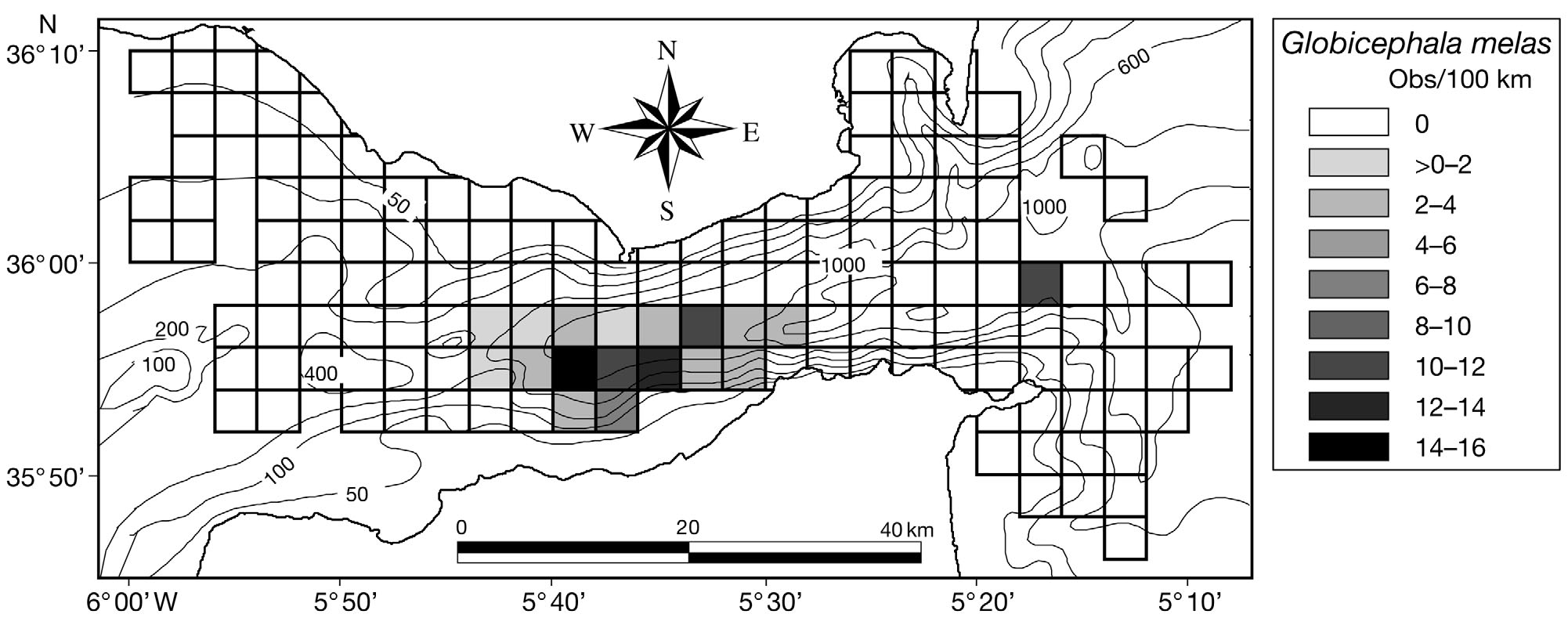Spatial autocorrelation ranges are given in kilometres structure (range) Delphinus delphis Exponential (1.3) Bottlenose dolphin Long-finned pilot whale Orcinus orca Bottlenose dolphins Tursiops truncatus were en- Pilot whales Globicephala melas and sperm whales countered in 10.0% of the quadrats sampled (Fig. 7).
Physeter macrocephalus were encountered in 12.0 Their presence was related to observation effort, and and 5.3%, respectively, of the quadrats sampled. The positively associated to steeper sea bottoms (linear distribution of both species was confined to the relationship, see Table 2). Bottlenose dolphins also southern parts of the study area (Figs. 8 & 9). Pilot tended to be found in the deeper areas, although whale data were too sparse to fit complex models the relationship was not or marginally significant accounting for the spatial autocorrelation of the data (p = 0.058).
(spatial models had very poor convergence and Fig. 5. Delphinus delphis. Distribution of encounter rates of common dolphins over the study area during this study

de Stephanis et al.: Summer distribution of cetaceans in the Strait of Gibraltar Fig. 6. Stenella coeruleoalba. Distribution of encounter rates of striped dolphins over the study area during this study Fig. 7. Tursiops truncatus. Distribution of encounter rates of bottlenose dolphins over the study area during this study Fig. 8. Globicephala melas. Distribution of encounter rates of long-finned pilot whales over the study area during this study Mar Ecol Prog Ser 353: 275–288, 2008 Fig. 9. Physeter macrocephalus. Distribution of encounter rates of sperm whales over the study area during this study residual diagnostics). Nevertheless, assuming spa- Spatial association–segregation between cetacean
tially independent data, we found a non-linear effect of depth on pilot whale presence (Table 2). Pilotwhales were less likely to be encountered in areas The standard deviations of the observed pairwise as- shallower than 300 m depth, and showed similar sociation indices were significantly higher than those preference for all depths between 300 and 800 m.
from permuted data (simple ratio index: p < 0.001; half- Sperm whale presence was positively and linearly weight index: p < 0.001), so the null hypothesis of a correlated to depth (Table 2).
random association in the space of species could be re- Killer whales Orcinus orca occurred in 7.2% of the jected. The cluster diagram (Fig. 12) and visual obser- quadrats sampled. They were encountered in the shal- vation of the distribution maps (Figs. 5 to 10) show that lower waters of the south-western part of the research 3 main groups of cetaceans can be distinguished. (1) area (Fig. 10). However, there was no statistically sig- Common dolphins and striped dolphins tended to be nificant relationship between killer whale presence spatially associated with each other. The overlap be- and depth or slope, probably owing to their low tween common dolphins and, to a lesser extent, be- encounter rate. However, visual comparison of killer tween striped dolphins and the other cetacean species whale sightings (Fig. 10) and tuna fishery (Fig. 11) was limited. (2) Bottlenose dolphins, long-finned pilot shows an unambiguously strong match.
whales and sperm whales shared a large part of their Fig. 10. Orcinus orca. Distribution of encounter rates of killer whales over the study area during this study de Stephanis et al.: Summer distribution of cetaceans in the Strait of Gibraltar Fig. 11. Distribution of sightings of tuna boats in the Strait of Gibraltar established from 2008 sampling stations (see ‘Materials this study. Most of these species areabundant, reaching an ER of between291.14 and 3.23 ind. per 100 km ofeffort for striped dolphins Stenellacoeruleoalba and killer whales Orcinusorca, respectively. Seven of the 9 spe-cies of cetaceans regularly seen in theMediterranean Sea (Reeves & Notar-bartolo di Sciara 2006) have beendescribed in the Strait of Gibraltar. Onemay suggest that the relatively highdiversity of cetacean species observedat the entrance of the MediterraneanSea could be related to a large number Fig. 12. Average-linkage cluster analyses of association (half-weight associ- of cetaceans transiting in and out of the ation index) between the different cetacean species in the Strait of Gibraltar Mediterranean Sea. However, long- (cophenetic correlation coefficient = 0.90) term, photo-identification work indi-cates that individual sperm whales Phy- habitat within the strait. (3) The smallest overlap with seter macrocephalus, pilot whales Globicephala melas, any other cetacean species was observed for killer bottlenose dolphins Tursiops truncatus, killer whales whales. All species but fin and killer whales were in- O. orca and common dolphins Delphinus delphis at volved in multi-species sightings (Table 1). A total of least are resident in the strait in summer (de Stephanis 15% of the sightings of the striped dolphins was seen unpubl. data), while the status of striped dolphins S. with common dolphins, and 14% of the sightings of coeruleoalba needs to be studied. Reul et al. (2002) common dolphins was seen with striped dolphins; 11 estimated that 5570 t C d–1 were transported towards and 4% of the sightings of long-finned pilot whales the Mediterranean Sea, while 1140 t C were exported were seen with bottlenose dolphins and sperm whales, daily towards the Atlantic by the deep Mediterranean respectively, representing 22 and 4% of the sightings of outflow. The strait is characterised by mixing processes bottlenose dolphins and sperm whales, respectively.
through a pulsed upwelling induced by the tides andconstrained by the strait's bathymetry (Echevarría etal. 2002). These phenomena are reflected in the boil- ing-water phenomena, occurring close to the KamaraRidge, and that produce vertical advection and mixing The Strait of Gibraltar is characterised by 7 species of processes (Bruno et al. 2002). The area is then a highly cetaceans, which were observed within the scope of productive area, and the most likely hypothesis to Mar Ecol Prog Ser 353: 275–288, 2008 explain the high density of cetaceans is prey availabil- cephalopods feeding on zooplankton are also sup- ity being enhanced within the Strait of Gibraltar.
ported. Diving studies of common dolphins and 2 In this study, data were pooled over 4 yr in order to Stenella species have shown that most dives are shal- produce statistically robust habitat –cetacean models.
lower than 150 m (Davis et al. 1996). This suggests that As a consequence, we only examined the static deter- both common dolphins and striped dolphins are likely minants of cetacean distribution, i.e. bathymetric to restrict most, if not all, of their feeding activity to the characteristics, which do not change from one year to layer of inflowing Atlantic waters. Furthermore the another. In this context, pooling the distribution data Atlantic–Mediterranean water interface may act as a over several years should have reduced the noise due boundary for their fish and squid prey and, as this to unknown environmental fluctuations and provided interface is shallower in the northern part of the strait, more robust relationships with bathymetry. In fact, it may enhance their foraging success in this area.
where the analyses could be run on individual years, Within the second group of cetaceans, pilot whales unstable results emerged, which could be attributed and sperm whales are known to be mainly squid eaters to insufficient data available. With temporally ‘aver- (Desportes & Mouritsen 1993, Gannon et al. 1997, aged' data, the spatial correlations we detect are Santos et al. 1999) and deep divers (Watkins et al.
unlikely caused by short-term spatial interactions such 1993, Baird et al. 2002). Thus, the spatial summer as conspecific attraction, but may rather reflect distribution of these 2 species within the strait is likely the spatial structures generated by un-modelled envi- to be indicative of the distribution of larger squid ronmental factors.
species encountered in the strait. However, it is Three distinct groups of species were identified unclear why bottlenose dolphins, which are mainly according to their distribution within the strait. Com- piscivorous (Barros & Odell 1990, Gannier 1995), mon and striped dolphins had a larger, broader distrib- tend to be spatially associated with sperm whales and ution and a preference for the northern part of the pilot whales.
study area, being mainly concentrated in deep waters Several diving studies on sperm whales have shown and along the north edge of the northern channel of that they dive regularly to depths >1000 m (Watkins et the Strait of Gibraltar (Figs. 5 & 6). Bottlenose dolphins, al. 1993), and, thus, they are able to reach the sea floor pilot whales and sperm whales shared a large part of throughout the study area. Interestingly, the ER of their foraging habitat, and were mainly found over sperm whale is higher just west of the Central Ridge, deep waters, over the main channel of the Strait of which separates the northern and main channels. The Gibraltar (Figs. 7 to 9). The third group included a sin- other area of higher ER of sperm whales is found east gle species: the killer whales, which were more com- of the Kamara Ridge. This suggests that sperm whales monly seen in the western part of the study area. The may forage in the deepest areas of the central strait.
differences in the spatial distribution between these 3 Pilot whales are also known to be relatively deep groups are likely related to their respective foraging divers, reaching depths between 200 and 600 m, with a ecology and, in particular, the fact that they are forag- maximum recorded depth of 828 m in the Ligurian Sea ing in different water masses.
(Baird et al. 2002). Pilot whales feed mainly on neritic There is little information on the diet of these species and oceanic squids and to a lesser extent on fishes that in the study area. According to other studies, both are most common at depths between 100 and 1000 m common and striped dolphins appear to be opportunis- (Desportes & Mouritsen 1993, Gannon et al. 1997).
tic feeders (Young & Cockcroft 1994, Gannier 1995), However, these prey exhibit vertical movements that targeting mainly small neritic fishes and cephalopods.
may allow the pilot whales to catch them at night, The small meso-pelagic cephalopods and myctophids when they are closer to the surface, while they may be tend to be higher diet components for the striped dol- inaccessible during the day (Desportes & Mouritsen phins (Blanco et al. 1995, Santos et al. 1996) than for 1993, Baird et al. 2002). The spatial distribution in sum- the common dolphins (Young & Cockcroft 1994, Santos mer of long-finned pilot whales and sperm whales et al. 1996). These differences may contribute to the indicates that both species are likely to exploit occurrence of striped dolphins over deeper waters squids — and possibly fishes — associated with the compared to common dolphins. Interestingly, both deep outflow of Mediterranean waters.
species are more abundant in the northern part of the Bottlenose dolphins present a similar distribution to strait, where enriched Atlantic Spanish shelf waters sperm whales. However, their dives are usually are circulating (Van Geen & Boyle 1988) and where between 10 and 50 m (Hastie et al. 2006). Therefore, plankton biomass concentration is higher and current they are likely to restrict their feeding to the surface velocities are lower than in the central and southern Atlantic water inflow. Bottlenose dolphins are oppor- parts of the strait (Reul et al. 2002). These ecological tunistic feeders and are considered to have a diet conditions may be more favourable for fishes, but small mainly based on demersal prey (Barros & Odell 1990, de Stephanis et al.: Summer distribution of cetaceans in the Strait of Gibraltar Gannier 1995), which seems unlikely in our study is too small to observe non-linear relationships such as because of their distribution over very deep waters, thresholds or mid-range optima. However, there is lit- where pelagic feeding appears to be the only possible tle doubt that careful treatment of error dispersion and foraging strategy. As we lack information on their diet spatial autocorrelation were the main factors responsi- over the study area, we are unable to determine if they ble for the parsimony of our models. Both overdisper- are feeding mainly on the pelagic prey associated with sion and spatial autocorrelation tend to inflate Type I the deep Mediterranean outflow migrating to the sur- error, that is, make unimportant covariates appear face at night, or if they feed on the pelagic prey associ- unduly significant (Keitt et al. 2002, Redfern et al.
ated with the Atlantic water inflow or both.
2006). In the case of GAMs, this also tends to exagger- Killer whale distribution was the most distinctive ate the non-linearity of the relationships with covari- when compared to other cetacean species occurring ates. In fact, experiences during the development of within the strait. Killer whales were seen interacting our models confirmed that in this data set, overly com- with the drop line fishery for bluefin tuna migrating plex additive terms were very easy to obtain when fail- out of the Mediterranean Sea after the completion of ing to account for one or both of these features. As a breeding. The summer killer whale distribution is spa- consequence, we concur with Redfern et al. (2006) in tially closely associated with the location of that fish- that the error structure and non-independence of ery, which is concentrated east of the Kamara Ridge, the data (e.g. spatial autocorrelation) should be sys- for the Moroccan fleet, and in the pass between Monte tematically controlled in habitat –cetacean studies.
Seco and Monte Tartesos, for the Spanish fleet.
The frequency of fin whale sightings in summer is Acknowledgements. This work was co-funded by CIRCE very low and consistent with recent results indicating from 2001 to 2004, the Autonomous City of Ceuta in 2001 and that most of the fin whale observations take place from the Life Nature Project (LIFE02NAT/E/8610) between 2002and 2004. Special thanks are due to P. Sanchez from the fall to spring (de Stephanis unpubl. data). Further- ‘Centre Mediterrani d'Investigacions Marines i Ambientals more, the catches reported by Aguilar (2006) were (CSIC)' in Barcelona and Y. Cherel from CEBC-CNRS for made in the Atlantic Ocean (Gulf of Cádiz), between their comments on squid distribution in the Alborán Sea and 32 and 37° N, and not in the Strait of Gibraltar itself, so the Gulf of Cadiz. We are also very grateful to the CIRCE staff a high presence of this species in the study area was and assistants in the field, P. Gozalbes, E. Pubill, R. Estebanand M. Fernández Casado. Thanks also to A. Cañadas, E.
not expected.
Urquiola, D. Desmonts, A. Aguilar, Y. Yaget and R. Sagarmi- Research into producing reliable variance estimates naga for their help, support and comments. Many thanks also for spatial model predictions has been identified as a to all the whale watching companies present in the strait, priority for cetacean distribution studies (Williams et Tumares S.L., Whale watch España, Aventura Marina and al. 2006). One of the conditions for this is that the vari- FIRMM for their comments on this manuscript and their help ance in the data themselves is properly modelled.
at sea. This research was conducted using software Logger2000 developed by the International Fund for Animal Welfare The present study shows that it is possible to esti- (IFAW) to promote benign and non-invasive research.
mate habitat –cetacean models that account for the un-der- or over-dispersion of errors, as well as their spatialautocorrelation. However, in some cases, models could not be estimated, or could only be after some simplifi-cation (e.g. not including spatial autocorrelation, see Aguilar A (2006) Catches of fin whales around the Iberian Peninsula: statistics and sources. Joint NAMMCO/IWC pilot whale or sperm whale models in Table 2). Like- Scientific workshop on the catch history, stock structure wise, reducing the amount of data by fitting models for and abundance of North Atlantic fin whales. Document individual years often resulted in unreliable models SC/14/FW/17-SC/M06/FW17, International Whaling (e.g. fitting algorithms did not converge or residuals Commission, Reykjavik Baird RW, Borsani JF, Hanson MB, Tyack PL (2002) Diving grossly violated normality or homoscedasticity as- and night-time behaviour of long-finned pilot whales in sumptions). This suggests that despite the intensive the Ligurian Sea. Mar Ecol Prog Ser 237:301–305 observation effort and the relatively large number of Barros NB, Odell DK (1990) Food habits of bottlenose dol- sightings, our data set is near the minimum required to phins in the southeastern United States. In: Leatherwood estimate robust habitat –cetacean associations.
S, Reeves RR (eds) The bottlenose dolphin. AcademicPress, San Diego, CA, p 309–328 Interestingly, most of the relationships we found Bejder L, Fletcher D, Bräger S (1998) A method for testing asso- between cetacean presence (or abundance) and ciation patterns of social animals. Anim Behav 56:719–725 covariates were linear or had very simple non-linear Blanco C, Aznar J, Raga JA (1995) Cephalopods in the diet of shapes (e.g. pilot whale), in contrast with many other the striped dolphin Stenella coeruleoalba from the west-ern Mediterranean during an epizootic in 1990. J Zool studies using GAMs (e.g. Forney 2000, Ferguson et al.
Lond 237:151–158 2006, Williams et al. 2006). One possible explanation is Bruno M, Alonso J, Cózar A, Vidal J, Echevarría F, Ruiz J, that the range of depths found in the Strait of Gibraltar Ruiz-Cañavate A, Gómez F (2002) The boiling water phe- Mar Ecol Prog Ser 353: 275–288, 2008 nomena at Camarinal Sill, the Strait of Gibraltar. Deep- Manly BFJ (1994) Multivariate statistical methods: a primer.
Sea Res II 49(19):4097–4113 Chapman & Hall, New York Cañadas A, Sagarminaga R, de Stephanis R, Urquiola E, Piatt JF, Wetzel J, Bell K, DeGange AR and 5 others (2006) Hammond P (2005) Habitat preference modelling as a Predictable hotspots and foraging habitat of the endan- conservation tool: proposals for marine protected areas for gered short-tailed albatross (Phoebastria albatrus) in the cetaceans in southern Spanish waters. Aquat Conserv 15: North Pacific: implications for conservation. Deep-Sea Res Part II 53:370–386 Davis RW, Worthy GAJ, Wursig B, Lynn SK, Townsend FI Pinheiro JC, Bates DM (2000) Mixed-effects models in S and (1996) Diving behavior and at sea movements of an S-PLUS. Springer Verlag, New York Atlantic spotted dolphin in the Gulf of Mexico. Mar R Development Core Team (2006) R: a language and environ- Mamm Sci 12:569–581 ment for statistical computing. R Foundation for Statistical Davis RW, Fargion GS, May N, Leming TD, Baumgartner M, Computing, Vienna. Available at www.R-project.org Evans WE, Hansen LJ, Mullin K (1998) Physical habitat of Redfern JV, Ferguson MC, Becker EA, Hyrenbach KD and 15 cetacean along the continental slope in the north-central others (2006) Techniques for cetacean-habitat modeling.
and western Gulf of Mexico. Mar Mamm Sci 14(3): Mar Ecol Prog Ser 310:271–295 Reeves R, Notarbartolo di Sciara G (eds) (2006) The status and Desportes G, Mouritsen R (1993) Preliminary results on the distribution of cetaceans in the Black Sea and Mediter- diet of long-finned pilot whales off the Faroe Islands. Rep ranean Sea. IUCN Centre for Mediterranean Cooperation, Int Whal Comm Spec Issue 14:305–324 Echevarría F, García Lafuente J, Bruno M, Gorsky G and 15 Reul A, Vargas JM, Jiménez-Gómez F, Echevarría F, Garcia- others (2002) Physical–biological coupling in the Strait of lafuente J, Rodriguez J (2002) Exchange of planktonic bio- Gibraltar. Deep-Sea Res II 49:4115–4130 mass through the Strait of Gibralatar in late summer con- Ferguson MC, Barlow J, Fiedler P, Reilly SB, Gerrodette T ditions. Deep-Sea Res Part II 49:4131–4144 (2006) Spatial models of delphinid (family Delphinidae) Roussel E (1999) Les cétacés dans la partie orientale du encounter rate and group size in the eastern tropical Détroit de Gibraltar au printemps: indications d'écologie.
Pacific Ocean. Ecol Model 193:645–662 Master thesis, Ecole Pratique des Hautes Etudes, Mont- Forney KA (2000) Environmental models of cetacean abun- dance: reducing uncertainty in population trends. Biol Sanjuán A, Zapata C, Álvarez G (1994) Mytilus galloprovin- Conserv 14:1271–1286 cialis and M. edulis on the coasts of the Iberian Peninsula.
Gannier A (1995) Les cétacés de Méditerranée nord-occiden- Mar Ecol Prog Ser 113:131–146 tale: estimation de leur abondance et mise en relation de Santos MB, Pierce GJ, López A, Barreiro A, Guerra A (1996) la variation saisonnière de leur distribution avec l'écologie Diets of small cetaceans stranded NW Spain. ICES Comm du milieu. Master thesis, Ecole Pratique des Hautes Etudes, Montpellier Santos MB, Pierce GJ, Boyle PR, Reid RJ and 7 others (1999) Gannon DP, Read AJ, Craddock JE, Fristrup KM, Nicolas JR Stomach contents of sperm whales Physeter macro- (1997) Feeding ecology of long-finned pilot whales Globi- cephalus stranded in the North Sea 1990–1996. Mar Ecol cephala melas in the western North Atlantic. Mar Ecol Prog Ser 183:281–294 Prog Ser 148:1–10 SEC (Sociedad Española de Cetáceos) (1999) Recopilación, Gil de Sola L (1993) Las pesquerías demersales del Mar de análisis, valoración y elaboración de protocolos sobre Alborán (sur-Mediterráneo Ibérico), evolución en los últi- las labores de observación, asistencia a varamientos y mos decenios. Inf Tec Inst Esp Oceanogr 142:1–179 recuperación de mamíferos y tortugas marinas de Ginsberg JR, Young TP (1992) Measuring association las aguas españolas. Technical Report Sociedad Española between individuals or groups in behavioural studies.
de Cetáceos, Secretaria General de Medio Ambiente, Anim Behav 44:377–379 Ministerio de Medio Ambiente Español, Madrid Hastie GD, Wilson B, Thompson PM (2006) Diving deep in a Silvani L, Gazo M, Aguilar A (1999) Spanish driftnet fishing foraging hotspot: acoustic insights into bottlenose dolphin and incidental catches in the western Mediterranean. Biol dive depths and feeding behaviour. Mar Biol 148: Conserv 90:79–85 Van Geen A, Boyle E (1988) Atlantic water masses in the Hooge PN, Eichenlaub B (2000) Animal movement extension Strait of Gibraltar: inversion of trace metal data. In: to Arcview, Ver 2.0. Alaska Science Center — Biological Almazan JL, Bryden H, Kinder T, Parrilla G (eds) Semi- Science Office, U.S. Geological Survey, Anchorage, AK.
nario sobre la oceanografía física del Estrecho de Gibral- Available at www.absc.usgs.gov/glba/ gistools/index.htm tar. SECEG, Madrid, p 68–81 Watkins WA, Daher MA, Fristrup KM, Howald TJ, Nortobar- Keitt TH, Bjornstad ON, Dixon PM, Citron-Pousty S (2002) tolo di Sciara G (1993) Sperm whales tagged with Accounting for spatial pattern when modelling organ- transponders and tracked underwater by sonar. Mar ism–environment interactions. Ecography 25:616–625 Mamm Sci 9:55–67 Kinder TH, Parrilla G, Bray NA, Burns DA (1988) The hydro- Williams R, Hedley SL, Hammond PS (2006) Modelling distri- graphic structure of the Strait of Gibraltar. In: Almazan JL, bution and abundance of Antarctic baleen whales using Bryden H, Kinder T, Parrilla G (eds) Seminario sobre la ships of opportunity. Ecol Soc 11(1):1 oceanografía física del Estrecho de Gibraltar, Madrid, Wood SN (2006) Generalized additive models: an introduction with R. Chapman and Hall/CRC, Boca Raton, FL Lacombe H, Richez C (1982) The regime of the Strait of Young DD, Cockcroft VG (1994) Diet of common dolphins (Del- Gibraltar. In: Nihoul JCJ (ed) Hydrodynamics of semi- phinus delphis) off the south-east coast of southern Africa: enclosed seas. Elsevier, Amsterdam, p 13–73 Opportunism or specialization? J Zool Lond 234:41–53 Editorial responsibility: Otto Kinne (Editor-in-Chief), Submitted: December 31, 2006; Accepted: July 18, 2007 Proofs received from author(s): January 3, 2008

Source: http://circe.info/files/deStephanis2008.pdf