Microsoft word - 20110310 ap008 forced degradation study with ice.doc

Reaction Analytics Inc.
2711 Centerville Road Suite 5992
Wilmington, DE 19808
Application Note # 008
Forced Degradation Study

Summary:
The degradation of famotidine is studied under isothermal and nonisothermal conditions. For
isothermal testing the temperature was held constant as samples were drawn over time. Data
was required at several different isotherms in order to calculate the Activation Energy. With
the nonisothermal method the temperature was ramped across a temperature range as samples
were collected. The results for either temperature profile match with each other and with
results from literature
Work Flow:
• HPLC Method Development • Sample Prep • Sample Run • Data Acquisition • Data Analysis • Data Presentation
The steps from Sample Run through Data Presentation are automated with the
iChemExplorer™ on an Agilent HPLC. Ease of implementation and speed to results promise
to make the iChemExplorer™ an effective tool for the study of forced degradation in
chemical development and formulation.
Introduction:
Although stress testing has played a critical role in the drug development process, some have
called it an "artful science" with a diversity of approaches depending greatly on the
experience and backgrounds of the scientists who are conducting the studies [1].
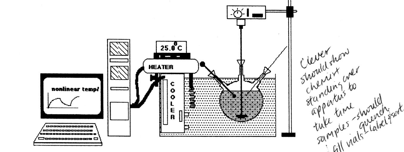
Investigators have heated samples in temperature controlled circulators [2] and ovens.
Figure 1: Water-bath set up for degradation testing with Chemist drawing samples 20110310 AP008 Forced Degradation Study with ICE
page 1 of 39

Reaction Analytics Inc.
2711 Centerville Road Suite 5992
Wilmington, DE 19808
All these techniques task the scientist with drawing samples and recording time and
temperature. Then the data must be assembled and computer algorithms applied [2] to
calculate thermodynamic properties. The iChemExplorer™ works with the HPLC to
automate the heating and sampling and then assembles the data for analysis and export to
Microsoft Excel for presentation and records.
Set Up:
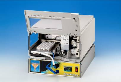
The iChemExplorer™ (ICE) hardware is designed to be compatible with the Agilent Model
1100 and 1200 Series HPLC systems. The electrically-heated ICE tray replaces the one-
hundred position vial tray in the 1313 and 1329 autosamplers (with gripper arm) and the 1367
well plate sampler (with needle in arm).

Figure 2: Image of Agilent HPLC autosampler with iChemExplorer™ ICEtray and ICEbox;
Inset of crimped vial with stir bar
The tray heats from ambient to 150 C with the temperature recorded and controlled through
the iChemExplorer™ software. The magnetic drive in the ICE Box under the autosampler
drives stir bars in the vials to 1200 RPM with manual control on the front of the box. The
configuration and operation of the HPLC remain unchanged. The system is suitable for
standard operation with either the ICEtray or Agilent tray in place.
The iChemExplorer™ software runs on the same PC that runs Chemstation software to drive
the Agilent HPLC. From the iChemExplorer™ home page create the sampling sequence,
record and control tray temperature and view and analyze data. Graphs and data are exported
as a report in Microsoft Excel for presentation and records
20110310 AP008 Forced Degradation Study with ICE
page 2 of 39 Reaction Analytics Inc.
2711 Centerville Road Suite 5992
Wilmington, DE 19808
Results:
The literature data for the degradation of famotidine is drawn from Reference [2] Here
solutions of famotidine were prepared with various pH buffers in 100 ml flasks. For the
sample run, each flask was placed in the open bath of a programmable circulator. The
temperature of the bath was raised at from 25 to 80 C at a rate of 0.375 C/min for a total ramp
time of four hours. Samples were drawn every ten minutes by the chemist and frozen to await
analysis. The samples were analyzed by HPLC and the thermodynamic values were
calculated from the data.

For Isothermal testing with the iChemExplorer™, the temperature of the heated tray was held
constant as samples were automatically drawn and analyzed by the HPLC from vials with
solution of famotidine and pH buffer. The tray temperature was stepped in this way from 25 C
to 55 C, 70 C and 85C. The Sample Run at each isotherm was extended to include three half-
lives of the starting material (approximately 12% remaining). The sample run time at 25 C
was almost twenty hours while a similar change in concentration took only twenty minutes at
85 C.
With Nonisothermal testing, the iChemExplorer™ drove the temperature of the heated tray
temperature from 25 C to 80 C over 720 minutes as samples were automatically drawn and
analyzed by the HPLC. Only a single set of vials was required to cover the same pH as the
Isothermal method above.
Effect of pH on Degradation:
The literature indicates that famotidine is stable in the middle of the pH range even at high
temperature as degradation proceeds at either high or low pH level. This effect of pH is
highlighted in an overlay of peak profiles from iChemExplorer™ for vials of famotidine at
pH 1, 4 and 10 that were sampled under nonisothermal conditions.
Figure 3: Overlay of peak profiles for pH 1 and pH 10 with difference in degradation product The peak profiles reconfirm the literature to show that pH level of the solution has a significant effect on the degradation pathway for famotidine. An overlay of data for pH 1 20110310 AP008 Forced Degradation Study with ICE
page 3 of 39 Reaction Analytics Inc.
2711 Centerville Road Suite 5992
Wilmington, DE 19808
onto data for pH 10 shows a significant difference in peak run time for the primary degradation product. In general the overall structures of the peak profiles are different. The degradation curves calculated by iChemExplorer™ to fit the data highlight the difference in pathway between High and Low pH levels. Figure 4: Overlay of degradation curves for famotidine with pH 1 and pH 10 buffers The curves show that at Low pH, famotidine begins to degrade at a lower temperature than at High pH but that the rate of degradation is slower. Effect of Organics Concentration on Degradation: For degradation testing, the API is dissolved in an organic solvent before dilution in aqueous solution with the pH buffer for testing. In the literature famotidine is first dissolved in methanol with the final concentration of methanol in water at two percent by volume. Higher concentration of organic solvent in the test solution is typical in commercial development as physical properties of a prospective API such as solubility is known as the time of testing. The integration of the iChemExplorer™ makes it possible to test different methanol concentrations in parallel with varying pH levels. The data fro the effect of methanol concentration on degradation is drawn from the data collected with Nonisothermal temperature ramp. 20110310 AP008 Forced Degradation Study with ICE
page 4 of 39 Reaction Analytics Inc.
2711 Centerville Road Suite 5992
Wilmington, DE 19808
Figure 5: Peak Profiles for famotidine degradation at pH10 with 2% and 30% v/v methanol Figure 6: Peak Profiles for famotidine degradation at pH1 with 2% and 30% v/v methanol This is further confirmed by an overlay of degradation curves. 20110310 AP008 Forced Degradation Study with ICE
page 5 of 39 Reaction Analytics Inc.
2711 Centerville Road Suite 5992
Wilmington, DE 19808
Figure 7: Overlay of degradation curves at high and low organics loading Figure 8: Overlay of degradation curves at high and low organics loading
As these graphs show, the higher concentration of methanol appears to depress degradation at
either pH level.
Results for Activation Energy:
The values for Activation Energy of famotidine from literature [2] and under Isothermal and
Nonisothermal temperature profiles are compiled in Figure Five. The values show close
agreement among the testing methods.
Source Data
Ea at low pH (KJ/mole)
Ea at High pH (KJ/mole)
Literature Nonisothermal [3] 70.4 @ pH 1.71 MeOH 2%
117.0 @ pH 10 MeOH 2%
Literature Isothermal [3] 67.2 @ pH 1.71 MeOH 2%
123.2 @ pH 10 Me OH 2%
68.1 @ pH 1 MeOH 2%
To be determined ICE Nonisothermal (ICE) 72.7 @ pH 1 MeOH 2%
118.10 @ pH 10 MeOH 2%
Figure 9: Table of Activation Energies for famotidine shows close agreement . 20110310 AP008 Forced Degradation Study with ICE
page 6 of 39 Reaction Analytics Inc.
2711 Centerville Road Suite 5992
Wilmington, DE 19808
Discussion:
The results from Nonisothermal degradation compare well with the results from Isothermal
testing. Nonisothermal testing brings shorter Sample Run Time, consumes less starting
material and provides data to calculate Activation Energy with shelf-life and rate constants at
temperature. The temperature range and ramp rate for the Nonisothermal ramp are selected
on the iHeat tab from the iChemExplorer™ home page. Selections in iHeat also provide the
flexibility in tray temperature control to pursue both Isothermal and Nonisothermal
degradation testing. So while Nonisothermal testing does offer advantages, Isothermal testing
is available as circumstances require.
The use of the iChemExplorer provides for consistent data collection with every sample run.
The chemist is freed from the tasks of drawing samples and maintaining records to devote his
effort interpreting what the data is saying. With the autosampler, the frequency and quality of
the samples are reproducible. The ICE software automatically records the tray temperature
with the time the sample is taken and then matches chromatographic data for a snapshot of
what's happening in each vial. Then iChemExplorer™ gives the tools to the chemist to
prepare the data for presentation and records while leaving the source data intact.
The iChemExplorer™ promises speed to results for chemical development. The learning
curve is short as the iChemExplorer™ builds on the knowledge and experience of an asset
already on most bench tops – the Agilent HPLC. The integration of heating and stirring with
sampling opens up the evaluation of dynamic chemistry in reaction kinetics, catalyst
screening, solvent screening and impurity generation. Fast and accurate results from this
work are critical to selecting those candidates to move forward

References:
1. KM Alsante, L Martin, SW Baertschi. A stress testing benchmarking study. Pharma
Tech. Feb 2003:60-72 2. MA Zoglio etal. Linear nonisothermal stability studies. J Pharma Sci. 57:2080-2085
3. GJ Junnarkar, S. Stavchansky. Isothermal and nonisothermal decomposition of
famotidine in aqueous solution. Pharma Res. 12:599-602 (1994) 4. M. Lee, S. Stavchansky. Isothermal and nonisothermal decomposition of Thymopentin
and its analogs in aqueous solution. Pharma Res. 15:1702-1707 (1998) 5. Z. Degim, I. Agabeyoglu. Nonisothermal stability tests of famotidine and nizatidine. Il
Farmaco. 57:729-735 (2002) 20110310 AP008 Forced Degradation Study with ICE
page 7 of 39 Reaction Analytics Inc.
2711 Centerville Road Suite 5992
Wilmington, DE 19808
SECTION II: Workflow Description:
The workflow presented here was developed to study of degradation of famotidine in solution
under isothermal and nonisothermal conditions. This workflow should be adaptable to the
study of any chemical of interest.
Workflow Steps
Description
HPLC Method Development Edit method, validate use and calibrate HPLC response Sample Preparation Prepare starting material solution and stressors Draw and analyze samples with iHeat in control of tray Data Acquisition Acquire source data from Chemstation data structure Apply iChem tools to refine how acquired data is shown Data Presentation Export data to Microsoft Excel for sharing and storage
Figure 10: Table of Workflow Steps for Study of Degradation
Operational Considerations:
HPLC Integration – The iChemExplorer™ ICE tray drops in place of the 100 position tray
to heat vials to 150 C in the Agilent 1100 and 1200 Series HPLC. The ICE box sits under the
HPLC autosampler to drive magnetic stir bars in the vials to 1200 RPM by manual control.
The iChemExplorer™ software works with Agilent Chemstation to acquire the data for
analysis and presentation. The HPLC continues to operate as before the installation. Agilent
Chemstation continues to drive HPLC operation.
Starting Material Requirements – The concentration of the starting material should be
dilute (less than 10 milligrams per milliliter) and fully soluble in solution. The starting
material may first be dissolved in an organic solvent that is also miscible with pH buffer and
other degradants such as methanol. As a milliliter is required per vial, a degradation run with
the iChemExplorer may use less than 50 milligrams total starting material.
System Maintenance - The design of the Agilent HPLC uses the flow of mobile phase to
wash all internal surfaces from pump through detector. The choice of mobile phase - optical
grade solvents such as methanol, acetonitrile and water – may be guided by the solubility of
the starting material and products to clear the system. This may be addressed in the Method
Development step of the work flow.
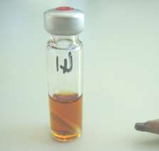
Vial Specification – A standard HPLC vial with silicone/PTFE septum in crimp top with 2X5
mm magnetic stir bar is recommended. Crimping provides a superior seal of septum to vial.
The silicone rubber in the septum holds up best to repeated piercing over a sample run and the
PTFE backing resists attack from organic solvents at temperature and extremes in pH.
Use of Internal Reference – The iChemExplorer™ makes the use of an internal reference
easy to incorporate into the workflow. Consider addition of Biphenyl to the solution as it is
widely available in high purity, slow to elute, stable under most temperature and chemical
conditions with high absorbance of UV light. Pick the reference peak from a drop down list
and iChemExplorer™ automatically corrects the concentration of the starting material.
20110310 AP008 Forced Degradation Study with ICE
page 8 of 39 Reaction Analytics Inc.
2711 Centerville Road Suite 5992
Wilmington, DE 19808
1. HPLC Method Development:
The following method was developed to determine concentration of famotidine in solution.
Parameter
Selection
Column Temperature Figure 11: Table of HPLC Method Parameters for Analysis of Famotidine in Solution By this method famotidine eluted at X.XX minutes. The method is optimized to minimize method run time to provide for more frequent sampling through the sequence. The Agilent Chemstation software provides Notes to consider when editing the method for use with iChemExplorer™: • Set Up Injector -.Select needle wash options; Select MORE to display draw and eject speeds as well as needle sample height adjustment.; Slow draw speed to 10 ul per minute; "0:" is 2.5 mm from bottom of vial with greater values raising the height from this zero point. • DAD Signals – Select multiple wavelengths to choose for best response • Signal Details – add signals for additional wavelengths so that data is recorded • Specify Report – Select File to activate types and Select CSV (integrated peak data) and EMF (image file of chromatograph); Select auto prefix to automate naming of injection folders in data subdirectory; Save the method to the Chemstation method folder. Choice of wavelength to collect chromatographic data - Looking for linear response over the range of interest. Consider use of a calibration table with concentration of starting material and reference if used at 100%, 87.5, 75% and 50%. Collect at wavelengths from 220 to 310 nm. Select a wavelength with best linear response over range and absorption with 20% to 80% of the detector range. 20110310 AP008 Forced Degradation Study with ICE
page 9 of 39 Reaction Analytics Inc.
2711 Centerville Road Suite 5992
Wilmington, DE 19808
2. Sample Prep:
Make up a stock solution of famotidine – [describe here – account for MeOH concentration]
Consider the addition of an internal reference material.
Prepare pH buffers.
[Any check of ionic strength of solution. The literature mentions that this value of solution
can have an affect on degradation rate.]
Prepare 2 ml vial by adding 1 ml of stock solution and X ml pH buffer. Add 2 X 5 mm
magnetic stir bar. Crimp top. Place vial in ICEtray and note position. For Isothermal
Temperature Profile then a set of vials must be prepared for each set point temperature while
only one set of vials is required for the Nonisothermal Temperature Profile.
20110310 AP008 Forced Degradation Study with ICE
page 10 of 39

Reaction Analytics Inc.
2711 Centerville Road Suite 5992
Wilmington, DE 19808
3. Sample Run:
For the Sample Run, iChemExplorer™ controls and records tray temperature while Agilent
Chemstation drives the HPLC to draw and analyze samples. The temperature of the tray is
controlled from the iHeat tab on the iChemExplorer™ home page. Manual and automatic
controls are provided to set the temperature profile. The Sequence Table in Chemstation sets
the sampling sequence. The Sequence Table may be created in iChemExplorer™ from the
iSample tab. Or it may be created directly in Chemstation. With the execution of the
Sequence Table, Chemstation is in control of the HPLC through the Sample Run.
With iHeat in control of the tray temperature, iChemExplorer™ records the time, tray
temperature and set point every twenty seconds to TEMPLOG.CSV and the time and tray
temperature for each sample drawn to the folder that holds the sample data.
3.1. Isothermal Temperature Profile:
With Isothermal control, the tray temperature is held constant through the sampling sequence.
See the Heat Table on the iHeat tab. The first entry by default is 22C at 0 elapsed minutes.
Enter the set point for the isotherm and the number of minutes to heat to this set point. Then
select Add Temp to populate these values to the Heat Table. This ramps the temperature of
the ICE tray to the set point. To hold the tray temperature at this set point, enter the set point
and the number of minutes to elapse at this set point and select Add Temp. In this way a Heat
Table is built to ramp and hold the tray temperature to a set point as sampling proceeds.
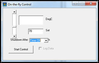
Figure 12: Add Temperature and Elapsed Time to Heat Table to control tray temperature An alternate method to set a constant set point is to select on-the-fly control on the iHeat tab. A window opens with a slider to select the set point. A shutdown timer is available with a drop down list to select the number of hours to run. 20110310 AP008 Forced Degradation Study with ICE
page 11 of 39

Reaction Analytics Inc.
2711 Centerville Road Suite 5992
Wilmington, DE 19808
Figure 13: iHeat on-the-fly control to manual control of tray temperature to a fixed set point Select Enable Log Data to record temperature through the Sample Run. This selection is required for iChemExplorer™ to record temperature when using on-the-fly control. 20110310 AP008 Forced Degradation Study with ICE
page 12 of 39

Reaction Analytics Inc.
2711 Centerville Road Suite 5992
Wilmington, DE 19808
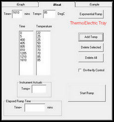
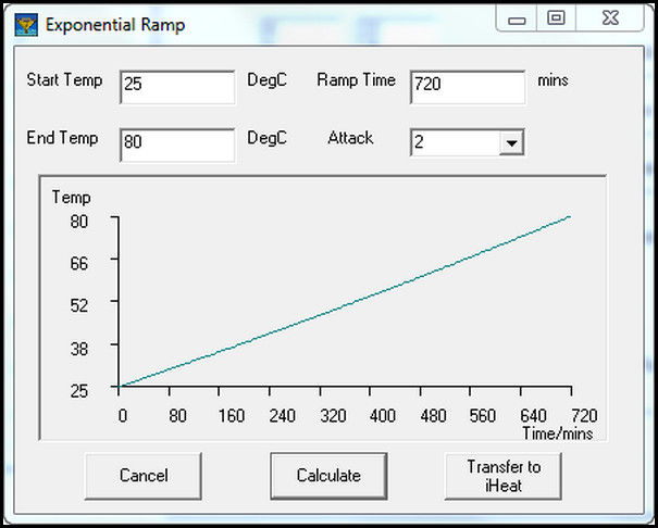
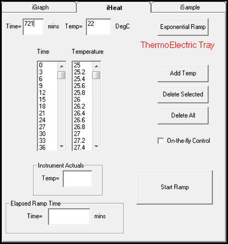
3.2. Nonisothermal Temperature Profile:
With nonisothermal temperature, the temperature of the tray is ramped over the duration of
the sampling sequence. To create a temperature ramp, select Exponential Ramp on the iHeat
tab. A window opens to enter the starting and ending temperatures with the ramp rate. To
enter the total time for the ramp instead of the ramp rate, select a value greater than one in the
Attack field. Enter the total ramp time in the field that has changed from ramp rate to time.
Select Calculate to show a graph of the temperature ramp in the window.
Figure 14: Use of Exponential Ramp to Generate Nonisothermal Temperature Profile Select Transfer to iHeat to populate the set point at three minute intervals to the Heat Table for automatic temperature control. Figure 15: Heat Table as populated by entries to Exponential Ramp 20110310 AP008 Forced Degradation Study with ICE
page 13 of 39

Reaction Analytics Inc.
2711 Centerville Road Suite 5992
Wilmington, DE 19808
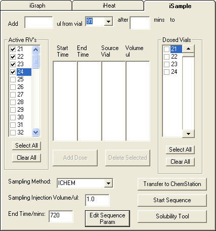
3.3 Sample Sequence:
The Sequence Table controls the operation of the HPLC through the Sample Run. The
procedure below describes the steps to generate a serial sampling sequence in Chemstation
from the iSample tab in iChemExplorer™. Start by selecting the analytical method from the
Sampling Method drop-down list. This list is populated from the Method folder in
Chemstation. Enter the sample volume. This volume is supersedes the sample volume in the
method. Enter the total time over which to sample from the vials
Figure 16: Use of iSample to create a serial sampling sequence in Agilent Chemstation Select the vial positions from the list of Active RV's (Reaction Vials) list. Figure 17: Double-click on RV selection to open Vial Description Window Double-click on the vial position to open a window to enter a Vial Description. These entries are automatically populated as the Sample Names in the Sequence Table. 20110310 AP008 Forced Degradation Study with ICE
page 14 of 39 Reaction Analytics Inc.
2711 Centerville Road Suite 5992
Wilmington, DE 19808
Select Edit Sequence Parameters to open the Sequence Parameters window in Chemstation. Enter a name and location for the data subdirectory to store the data from the sample run. Check that the Auto button is selected. With this selection Chemstation follows a specific format to name the sample folders stored to the subdirectory. iChemExplorer™ uses this naming convention to automate the acquisition of the data. Select OK to apply the entries and close the window. Figure 18: Create the Data Subdirectory and Name the Sample Data Folders in Chemstation On the iSample tab, select Transfer to Chemstation to generate the Sequence Table in Chemstation. Figure 19: Generation of Sequence Table in Chemstation with estimate for samples drawn Once complete, a window opens with an estimate of the number of samples per Reaction Vial. 20110310 AP008 Forced Degradation Study with ICE
page 15 of 39 Reaction Analytics Inc.
2711 Centerville Road Suite 5992
Wilmington, DE 19808
Go to Chemstation to view the Sequence Table. The table shows a serial sampling sequence. In this sequence, samples are drawn from the first through the last vials and then repeated for the length of the End Time entered into iSample. Figure 20: Sequence Table in Chemstation as populated by iSample in iChemExplorer™ iSample is used to generate new sampling sequences only. Make changes to the Sequence Table directly in Chemstation. 20110310 AP008 Forced Degradation Study with ICE
page 16 of 39 Reaction Analytics Inc.
2711 Centerville Road Suite 5992
Wilmington, DE 19808
3.4. Start and Stop Sample Run:
With iChemExplorer™, control of tray temperature is independent of HPLC operation for the
Sample Run. To start and stop temperature control, use the iHeat tab or the on-the-fly control
window. Select Start Ramp to initiate control. The button title changes to Stop Ramp to
indicate that control is underway. Changes to temperature control may be made during the
sample run in iHeat. Select Stop Ramp to end control. This selection ends the recording of
tray temperature for the run and resets the tray set point to 22 C.
Agilent Chemstation is in control of HPLC operation for the Sample Run. The Sequence
Table may be started from the iSample tab by selecting Start Sequence. The Sequence Table
may also be started directly in Chemstation. Go to the Sequence Table to make changes and
to end the sampling sequence.
20110310 AP008 Forced Degradation Study with ICE
page 17 of 39 Reaction Analytics Inc.
2711 Centerville Road Suite 5992
Wilmington, DE 19808
4. Data Acquisition
iChemExplorer™ software eases the acquisition of data generated through sample run. By
acquiring the data, iChemExplorer™ leaves the source data intact.
4.1 Data Structure:
iChemExplorer™ software uses the data structure created by Chemstation to store sample
data. Chemstation creates a subdirectory named in the Sequence Parameter window.
Chemstation then creates a folder to store the data for each sample injection in this
subdirectory. The selection of Auto on the Sequence Parameter window automatically names
the sample folder. The folder name follows the form of XXX-XXXX where the first three
positions indicate vial position from 001 to 100; the next two positions show the order of the
sample in the sequence in hexadecimal numbers; and the last two positions represent the
number of injection per sample.
Figure 21: Subdirectory contains TempLog with Sample Data Folders 4.2 Templog.CSV File When using iHeat to control tray temperature, iChemExplorer™ automatically records tray temperature and set point every twenty seconds to the Templog.csv file. Figure 22: Example of TempLog.CSV file 20110310 AP008 Forced Degradation Study with ICE
page 18 of 39 Reaction Analytics Inc.
2711 Centerville Road Suite 5992
Wilmington, DE 19808
This data may then be used to construct a time-temperature plot for the Sample Run. Chemstation records the method conditions to [file name]00.CSV. The method detail recorded to this file may be viewed in iChemExplorer™ from View>Detail Pane. The integrated peak data for each wavelength is recorded to [file name]0X.CSV where X is the order of wavelength collected according to the method. iChemExplorer™ records the tray temperature with the time the sample was drawn to [filename]99.CSV. Figure 23 – Data Structure from Sequence Run Chemstation stores an image of the sample chromatographs to [filename].EMF. 20110310 AP008 Forced Degradation Study with ICE
page 19 of 39 Reaction Analytics Inc.
2711 Centerville Road Suite 5992
Wilmington, DE 19808
4.2 Load HPLC Data To acquire the data into iChemExplorer™ select Load HPLC Data on the home page. A Windows Explorer window opens to navigate to the sample folders in the data subdirectory. Open any sample folder and select a CSV file with the integrated peak data. Figure 24: Windows Explorer is used to load data to iChemExplorer iGraph iChemExplorer™ software acquires the same filename as selected from each of the sample folders in the subdirectory. The vials positions with acquired data are shown in white on the tray graphic. 20110310 AP008 Forced Degradation Study with ICE
page 20 of 39 Reaction Analytics Inc.
2711 Centerville Road Suite 5992
Wilmington, DE 19808
4.3 Peak Profile Select a vial position in white to view the Peak Profile in the iGraph window. Figure 25: iGraph shows the degradation of famotidine by sample The lines of the Peak Profile follow the peaks from sample to sample 20110310 AP008 Forced Degradation Study with ICE
page 21 of 39 Reaction Analytics Inc.
2711 Centerville Road Suite 5992
Wilmington, DE 19808
4.4 Viewing Chromatographs To see the underlying chromatographic data, place the cursor on the iGraph window and left-click. A window opens to view the chromatographs. The vial position on view is shown in the title bar of the window. Figure 26: View the chromatographs for each vial with Copy and Paste Functions Select Previous and Next to page through the chromatographs by vial position. Select Scroll to automatically display one graph after another like a movie for that vial position. Select Previous Sample and Next Sample to see graphs for other vial positions. Select Copy to Clipboard to copy and paste chromatographs to any Windows-compatible application. Now we are on to making sense of this acquired data using the tools in iChemExplorer™. 20110310 AP008 Forced Degradation Study with ICE
page 22 of 39 Reaction Analytics Inc.
2711 Centerville Road Suite 5992
Wilmington, DE 19808
5. Data Analysis
iChemExplorer™ provides tools to better view the acquired data and to calculate the
degradation properties of the starting material. iGraph is a window on the acquired data to
view changes as they are made. The integrated data as acquired is first displayed as a Peak
Profile – lines assigned by peak run time that follow area percent for that peak from sample to
sample.
5.1 Peak Locator
The values for the parameters in the Peak Locator section on the iChemExplorer™ home page
guide the assignment of peaks to display on the Peak Profile. The boundaries managed by
these parameters are described here.
• Threshold – Minimum peak height required to assign a peak profile relative to the maximum peak height across all vial positions. Higher values set a higher bar for peaks to meet in order for a peak profile to be assigned. • Tolerance – Maximum difference in peak run time over which to group peaks from one sample to the next. Higher values set a wider band to group peak run times to assign to a single peak profile. • Range – Set the range in run time across which to assign peak profiles. Peak run- times before the Minimum and after the Maximum are excluded from presentation. The values for the Peak Locator parameters are populated from default entries under File>Preferences. See Appendix A for more information about how to set preferences. As applied to the acquired data, something looks wrong with the Peak Profile. Figure 27: Peak Profile in iGraph Window at Low Tolerance Value The Remainder – the difference in peak area after all assigned peaks are subtracted – follows the expected consumption of the starting material as degradation proceeds. The value for Threshold includes the peaks for significant degradation byproducts. Time Range includes the peak run times for the starting material and the byproducts. 20110310 AP008 Forced Degradation Study with ICE
page 23 of 39 Reaction Analytics Inc.
2711 Centerville Road Suite 5992
Wilmington, DE 19808
Let's look at the chromatographs with the iGraph Viewer. The value for Threshold would account for this Remainder at 3 % is a tight window with only 0.06 minutes on either side of the peak run-time for the starting material at 2.08 minutes. The peak run-time for the starting material shifts from 1.89 minutes at the beginning of the sample run to 2.08 minutes at the end for a total shift of 0.19 minutes or 9.1% of the peak-run time. Figure 28: See shift in peak run-time for starting material from first to last chromatograph With Tolerance increased to 10% in order to account for the shift, the Peak Profile now better represents the underlying chromatographic data. Figure 29: Increase in Tolerance accounted for shift in peak run-time 20110310 AP008 Forced Degradation Study with ICE
page 24 of 39 Reaction Analytics Inc.
2711 Centerville Road Suite 5992
Wilmington, DE 19808
5.2 Peak Edit iChemExplorer™ provides an editor to hide, name and color Peak Profile lines. From the top bar select Edit and then select Peak Names from the list. A window opens that lists the assigned peaks by run-time. Figure 30: Edit Peak Names from the Sample Run Rename peaks by entering a name in the associated field. Change the peak color by selecting Recolor and choose the color from the drop-down list. Options are provided to normalize visible peak areas upon selection to hide a peak. 20110310 AP008 Forced Degradation Study with ICE
page 25 of 39 Reaction Analytics Inc.
2711 Centerville Road Suite 5992
Wilmington, DE 19808
5.3 Data Point Exclusion iChemExplorer™ provides for the selection of sample data to exclude from the acquired data to be presented. The sample data for the selected vial position are listed in the Exclude window on the iChemExplorer™ home page. Figure 31: Exclude sample data from the Data Presentation Select and deselect sample data from this list to exclude or include in the acquired data. Sample data excluded here is also excluded from Data Presentation. 20110310 AP008 Forced Degradation Study with ICE
page 26 of 39 Reaction Analytics Inc.
2711 Centerville Road Suite 5992
Wilmington, DE 19808
5.4 iGraph Overlay Mode iChemExplorer™ provides the ability to overlay the graphs shown in the iGraph window. To start a graph is already shown in the iGraph window for the selected vial position. Select Enable Overlay Mode above the tray graphic on the iChemExplorer™ home page. Then select another vial position to overlay on the graph already in the window. Figure 32: Select Enable Overlay Mode and select vial positions to overlay Peak Profiles To eliminate the overlay, deselect the Overlay Mode. Then select a vial position from the tray graphic. The iGraph window only shows the graph for the newly selected position. Select Copy Graph to Clipboard to paste the overlay to any Windows-compatible application.
20110310 AP008 Forced Degradation Study with ICE
page 27 of 39 Reaction Analytics Inc.
2711 Centerville Road Suite 5992
Wilmington, DE 19808
5.5 Degradation Profile iChemExplorer™ uses the data acquired in nonisothermal testing to calculate the degradation properties of the Starting Material. Start with the Peak Profile for the selected vial position in the iGraph window. See that the Plot selection under the iGraph window shows Area %. The calculation of degradation properties comes with the choice to display the degradation results in the iGraph window. Figure 33: Select the Peak for the starting material from the drop down list Select Degradation from the Plot drop-down list. A window opens to select the peak for the starting material. Choose the peak for starting material from the drop down list. Select OK to proceed to build the degradation graph in the iGraph window. 20110310 AP008 Forced Degradation Study with ICE
page 28 of 39 Reaction Analytics Inc.
2711 Centerville Road Suite 5992
Wilmington, DE 19808
5.7 Axis Set-Up The window in iGraph now shows the concentration of the starting material on the y-axis with sample on the x-axis. The graphs may be brought together by substituting temperature for the x-axis. Figure 34: Degradation Curve with Samples on x-axis In the Axis Set-Up section, select Temperature for the x-axis. The graph now uses the common axis to overlay the degradation curve on the sample data Figure 35: Degradation Curve with Common Temperature Axis 20110310 AP008 Forced Degradation Study with ICE
page 29 of 39 Reaction Analytics Inc.
2711 Centerville Road Suite 5992
Wilmington, DE 19808
The Degradation Curve as fitted to the sample data is displayed in the iGraph window. The graph below was pasted here using the Copy button in iChemExplorer™. Above the graph are values for quality of fit, Activation Energy and Intercept. Figure 36: Degradation Curve with highlights on Error and Activation Energy Values The Activation Energy is provides in KJ/mole. Multiply by 4.185 to convert to Kcal/mole. The quality of fit for the degradation curve to the experimental data is indicated by the RMS Error value. Lesser values indicate better quality of fit. Changes to fit may be made by excluding data points as described earlier. Compare the results 20110310 AP008 Forced Degradation Study with ICE
page 30 of 39 Reaction Analytics Inc.
2711 Centerville Road Suite 5992
Wilmington, DE 19808
5.8 Save Analysis The analysis as described may be saved as an ICE file. This file type stores the values set through data analysis with a map to the source data. Go to the top bar on the iChemExplorer™ home page. Select File and then select Save Analysis from the menu items. Figure 37: Select File>Save Analysis to create iChem file to load data with analysis A Windows Explorer window opens to locate and name the file. See that the file type is .ICE. Opening this file automatically acquires the source data into iChemExplorer™ and populates the settings from the analysis to duplicate the presented results. 20110310 AP008 Forced Degradation Study with ICE
page 31 of 39 Reaction Analytics Inc.
2711 Centerville Road Suite 5992
Wilmington, DE 19808
6. Data Presentation:
The data as analyzed is now ready for export. iChemExplorer™ provides templates to export
the data. Go to the top bar on the iChemExplorer™ home page and select Reports. On the
menu see the following selections – Collated, Solubility, Degradation and Area by Time.
Description
Peak Profiles by Area Graph for each vial position by peak area Peak Profiles by Area % Graph for each vial position by peak area % First, middle and last chromatographs as included with Collated
Graph of temperature and set point over time Collated Data by Area Spreadsheet with all data in numerical form by area Collated Data by Area % Spreadsheet with all data in numerical form by area % Graph for each vial position with calculation of half Degradation Profiles life and rate constant First, middle and last chromatographs as included with Degradation
data analysis Spreadsheet of all data included in numerical form by Degradation Data Figure 38: Table of tabs for Excel export Reports available through iChemExplorer 20110310 AP008 Forced Degradation Study with ICE
page 32 of 39 Reaction Analytics Inc.
2711 Centerville Road Suite 5992
Wilmington, DE 19808
6.1 Collated Report Select Collated to export the Peak Profiles for each vial position. A Windows Explorer window opens to locate and name the Microsoft Excel file. A window opens to show the progress in exporting the report. Figure 39: Selected Tabs from Excel export of Collated Report Open the Microsoft Excel workbook for the Collated Report. The first two tabs provide Peak Profiles for each vial by peak area and peak area percent. The third tab includes images of the first, middle and last chromatographs as included in the data analysis. The fourth tab is a chart of temperature and set point over time as recorded with iHeat. The fifth and sixth tabs list the numeric data as included in the data analysis. 20110310 AP008 Forced Degradation Study with ICE
page 33 of 39 Reaction Analytics Inc.
2711 Centerville Road Suite 5992
Wilmington, DE 19808
6.2 Degradation Report For the Degradation Report select Degradation from the Report menu. Windows Explorer opens to locate and name the file. Select Open to initiate the export. Windows open to show progress. Once complete then open the report in Microsoft Excel. Figure 40: Tabs for Degradation Report as exported to Microsoft Excel See three tabs for worksheets in the report. The first tab includes triple-axis graphs to copy and paste with calculated data including Activation Energy for each vial position. The second tab provides images of the first, middle and last chromatograph as included in the data analysis to copy and paste. The third tab lists the numerical data as included in the data analysis for further study. 20110310 AP008 Forced Degradation Study with ICE
page 34 of 39 Reaction Analytics Inc.
2711 Centerville Road Suite 5992
Wilmington, DE 19808
6.3 Triple Axis Graph The Degradation Report provides a triple-axis chart that integrates the experimental data for a nonisothermal degradation study. Vial # 42 (Exp. Name Fam pH1 2% MeOH)
Figure 41: Degradation Curve fit to Nonisothermal Degradation of Famotidine at pH 1 The chart shows starting material concentration on the y-axis at the left. Time is shown on the x-axis at the bottom. Temperature is shown on the y-axis to the right. The green line follows the degradation curve that best fits the sample data as shown in yellow triangles. The red line follows the temperature over the sample time. In this way the temperature ramp may be viewed on the same graph as the degradation curve for a complete picture of what's going on in the vial. Vial # 46 (Exp. Name Fam pH10 2% MeOH)
0 Time/h 5
Figure 42: Degradation Curve Fit to Nonisothermal Degradation of Famotidine at pH 10 The same triple axis chart for famotidine at pH 10 highlights the slower degradation rate under basic conditions. 20110310 AP008 Forced Degradation Study with ICE
page 35 of 39 Reaction Analytics Inc.
2711 Centerville Road Suite 5992
Wilmington, DE 19808
Addendum A: Setting Preferences in iChemExplorer™
The default values for these parameters are set in the Preferences window opened from File
on the top bar of the iChemExplorer™ home page.
Figure 43: Select Excel Export to set the defaults for how graphs are exported Select the INI tab to enter new default values. Select Apply to set the new values on the home page and close the Preferences window. Figure 44: Select .ini Settings to assign default values for Peak Locator and method 20110310 AP008 Forced Degradation Study with ICE
page 36 of 39 Reaction Analytics Inc.
2711 Centerville Road Suite 5992
Wilmington, DE 19808
The Degradation Report includes values calculated for various temperatures. The standard default is 25, 50, 75 and 100 C. The defaults for these values may be rest on the Degradation tab. Figure 45: Set Temperature Values for Thermodynamic calculations in Degradation Report 20110310 AP008 Forced Degradation Study with ICE
page 37 of 39 Reaction Analytics Inc.
2711 Centerville Road Suite 5992
Wilmington, DE 19808
Addendum B: Experiment Design
Create a Microsoft Excel spreadsheet to define the design on the experiment. There are only
two requirements for the spreadsheet
Figure 46: Create Excel file to record vial conditions for the experiment The first requirement is that top row (1) is reserved for variable identifiers. You may include as many variables as you wish. The second requirement that the first column (A) lists the vial positions with data starting in the second row. Figure 47: Select Add Design to open Window to apply Experiment Design 20110310 AP008 Forced Degradation Study with ICE
page 38 of 39 Reaction Analytics Inc.
2711 Centerville Road Suite 5992
Wilmington, DE 19808
Figure 48: With Experiment Design Color By: and Reaction Details are active With this design you will see the variable identifiers with values for the selected vial position in the window on the home page. You may select a variable identifier from the Color by: drop down menu to color those positions by variable value. 20110310 AP008 Forced Degradation Study with ICE
page 39 of 39

Source: http://www.ichemexplorer.com/ApNotes/FDApNote